Simulation of modelling and control for aircraft pitch毕业论文
2020-04-15 21:04:50

毕业设计(论文)任务书
课题名称 | Simulation of modelling |
and control for aircraft pitch | |
院 (系) | 电气工程与控制科学学院 |
专 业 | 自动化(留学生) |
姓 名 | Aibek Ablay |
学 号 | L1501150233 |
指导教师 | 沈谋全 |
起讫日期 | 2019.06 |
2019年 6月 |
Simulation of modeling and control for aircraft pitch
Abstract
This paper gives an overview of the aircraft control system, a graphical software environment for the design and analysis of the aircraft dynamics control system based upon MATLAB and SIMULINK. Its main purpose is to simplify the design process of the flight control system
It uses Bode plots and root plots to determine stability characteristics based on time domain and frequency domain. The aircraft takes an eclectic approach for parameter identification method. The time domain method for estimating stability control parameters is used in conjunction with the frequency domain method, which is primarily used to determine flight quality parameters. Stability is an important factor in Aircraft It is important to understand the various stability factors before making comments on aircraft stability. As part of this project, we envisioned a fly-by-wire aircraft, a semi-automatic aircraft, usually a computer established system used to control the flight of an aircraft or spacecraft. The system identification method is based on the input and output measurements of the dynamic system to form a mathematical model or a series of models. These extracted models make it possible to characterize the response of the aircraft or the general behavior of the components and to record constant values or changes. System identification is the process used to accurately characterize the dynamic response behavior of a completed aircraft and its response to the control system. This technology for the development and integration of modern fly-by-wire flight control systems provides a unified flow of information about system performance. The values obtained from the mathematical model. Models can be defined in two ways using time domain analysis, the root locus technique and frequency domain analysis using bode plot technique.
The use of complex mathematical calculations to determine aircraft stability generally requires time and approximation consideration. In this project, the stability of an aircraft such as Boeing 767 was analyzed. The stability factors are determined by the state space model in the MATLAB (Simulink) software. Using the software to determine the stability simplifies work and reduces time. This gives more precise values and the results are more convincing.
Keywords: pitch angle, angle of attack, state-space, state feedback, pole placement.
Contents
- System Modeling
- Physical setup and system equations
- Transfer function and state-space models
- Design requirements
- MATLAB representation
- System Analysis
- Open-loop response
- Closed-loop response
- PID controller design
- Proportional control
- PI control
- PID control
- Root Locus controller design
- Original root locus plot
- Lead compensation
- Frequency Domain Methods for Controller Design
- Open-loop response
- Closed-loop response
- Lead compensator
- State-Space Methods for Controller Design
- Controllability
- Control design via pole placement
- Linear quadratic regulation
- Adding pre-compensation
- Digital controller design
- Discrete state space
- Controllability
- Control design via pole placement
- Adding pre-compensation
- Simulink Modeling
- Physical setup and system equations
- Building the state-space model
- Generating the open-loop and closed-loop response
- Simulink controller design
- State-space feedback with pre-compensation
- System robustness
- Automated PID tuning with Simulink
Conclusion
Acknowledgement
Reference
Chapter 1
Problem Statement and Overview
The equation governing aircraft motion is a very complex set of six nonlinear coupled differential equations. However, under certain assumptions, they can be decoupled and linearized into longitudinal and lateral equations. The pitch of the aircraft is determined by the longitudinal dynamics. These equations form an unstable system that, in addition to stabilizing the system, requires the controller to achieve the required accuracy in a reasonable amount of time.
In this project, we used MATLAB and Simulink modeling to design an autopilot that controls the pitch of the aircraft. The PID tuner is designed using the MATLAB Control Designer to stabilize the system and provide the desired results (to meet certain predefined design requirements). Finally, the Simulink model of the system was developed and the system performance was tested.
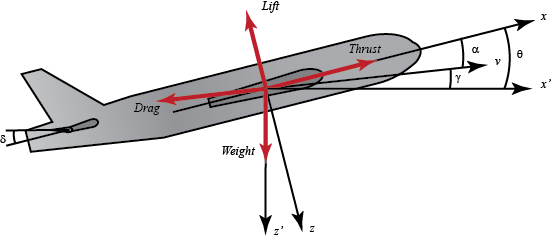
We will assume that the aircraft is in steady-cruise at constant altitude and velocity; thus, the thrust, drag, weight and lift forces balance each other in the x – and y -directions. We will also assume that a change in pitch angle will not change the speed of the aircraft under any circumstance (unrealistic but simplifies the problem a bit).
1. Introduction
Flight dynamics the study of the motion of an aircraft or missile; concerned with transient or short-term effects relating to the stability and control of the vehicle, rather than to calculating such performance as altitude or velocity. The three critical flight dynamics parameters are the angles of rotation in three dimensions about the vehicle's center of mass, known as roll, pitch and yaw [1].
- Aircraft Pitch: System Modeling
1.2 Physical setup and system equations
The equations governing the motion of an aircraft are a very complicated set of six nonlinear coupled differential equations. However, under certain assumptions, they can be decoupled and linearized into longitudinal and lateral equations. Aircraft pitch is governed by the longitudinal dynamics. In this example we will design an autopilot that controls the pitch of an aircraft.
The basic coordinate axes and forces acting on an aircraft are shown in the figure given below.
1.3 Physical System
The linearized equations of motion under the aforementioned assumptions are as follows:
= µΩϭ[ - (CL CD)α µ = q – (CW sinγ)θ CL ]
= [[CM - ƞ(CL CD)]α [CM ϭCM(1 - µCL)]q (ƞCWsinγ)δ]
= Ωq
where,
α= Angle of attack.
q = Pitch rate.
θ = Pitch angle.
δ = Elevator deflection angle.
µ = .
p = Density of the air.
S = Platform area of the wing.
= Average chord length.
m = Mass of the aircraft.
Ω = .
U = Equilibrium flight speed.
CT = Coefficient of thrust.
CD = Coefficient of drag.
CL = Coefficient of lift.
CW = Coefficient of weight.
CM = Coefficient of pitch moment.
γ = Flight path angle.
ϭ = = Constant.
= Normalized moment of inertia.
ƞ = µϭCM = Constant.
System Modelling
Considering the values taken from the data from one of Boeing's commercial aircraft`s, the system equations can be written with numerical coefficients as follows:
= -0.313α 56.7q 0.232δ
= -0.0139α – 0.426q 0.0203δ
= 56.7q
For this system, the input will be the elevator deflection angle and the output will be the pitch angle of the aircraft. We will plug in some numerical values in our equations taken from the data from one of Boeing's commercial aircraft [3].
Subsequently, the state-space model of the system can be made, with the state variables and external input
y =
The output for this system is the pitch angle, thus the open loop transfer function, computed by taking the Laplace transform of the system equations and performing certain mathematical manipulations, is
P(s) = =
Transfer function
To find the transfer function of the above system, we need to take the Laplace transform of the above modeling equations. Recall that when finding a transfer function, zero initial conditions must be assumed. The Laplace transform of the above equations are shown below:
sA(s) = -0.313A(s) 56.7Q(s) 0.232∆(s)
sQ(s) = -0.313A(s) – 0.426Q(s) 0.0203∆(s)
s(s) = 56.7Q(s)
Then we obtain following transfer function :
P(s) = =
2.2 Open Loop Response
The step response of the open loop system is as follows
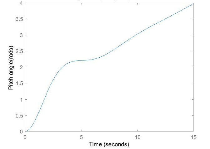
Figure:1.3 Open - loop step response
It can clearly be seen that this system is unstable. The system has a pole on the origin, which acts a pure integrator. Therefore, when the system is given a step input its output continues to grow to infinity.
2.3 Closed Loop Response
The unity gain closed loop transfer function of the system is as follows
Y(s) = R(s)
Corresponding to this, the step response of the system is
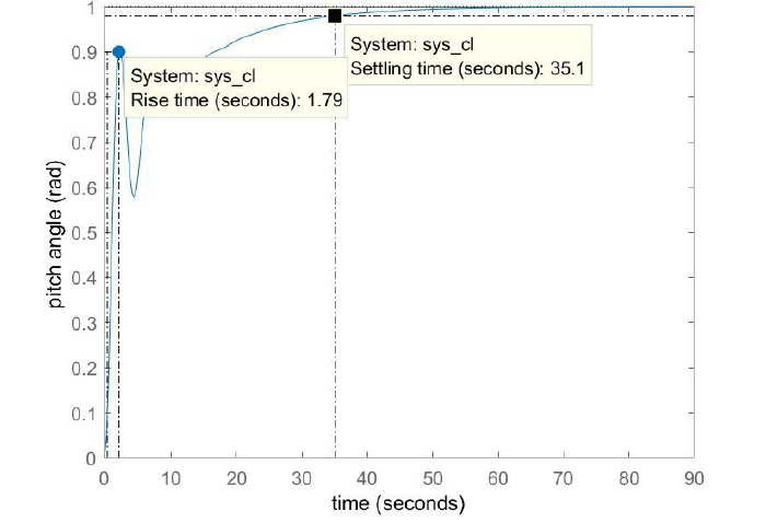
Figure:1.4 Closed – loop step response
While the closed loop system is stable, it can be seen that this system is very sluggish in terms of the settling time and also has a sharp oscillatory behaviour immediately following its initial rise. In order to improve the performance of this system, a controller is designed which meets the following design specifications:
Overshoot less than 10%
Rise time less than 2 seconds
Settling time less than 10 seconds
Steady-state error less than 2%
- PID Controller Design
Step 1 - Proportional Control:
We have used the MATLAB Control System Designer tool to tune the controller. We started off by adding a simple proportional controller.
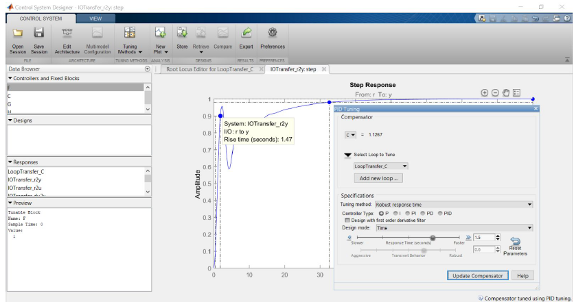
This controller meets the rise time requirement, but the settle time is much too large. A faster response time can be acquired by moving the slider to the right, however, this will result in an increase in overshoot and oscillation. The proportional controller does not provide a sufficient degree of freedom in tuning. Since the steady state requirement is already met, we will directly move to a PID Controller rather than a PI Controller.
Step 2 - PID Control:
By adding derivative control, we may be able to reduce the oscillation in the response a sufficient amount that we can then increase the other gains to reduce the settling time.
Transfer Function for PID Controller
1.8576
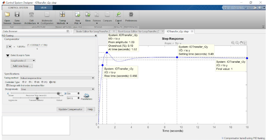
Reducing the Response Time requirement (moving the slider to the right) will make the response faster.
Moving the Transient Behavior slider towards Robust will help reduce the oscillation.
This response meets all of the requirements. So this is our final PID Controller.
Lead Controller Design
This is the original root locus design:
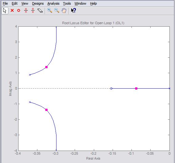
Settling time, Percent overshoot can be added directly. Rise time is not explicitly included as one of the drop-down choices, however, we can use the following approximate relationship that relates rise time to natural frequency.
Therefore, our requirement that rise time be less than 2 seconds corresponds approximately to a natural frequency of greater than 0.9 rad/sec for a canonical underdamped second-order system. Adding this requirement to the root locus plot in addition to the settle time and overshoot requirements generates the following figure.
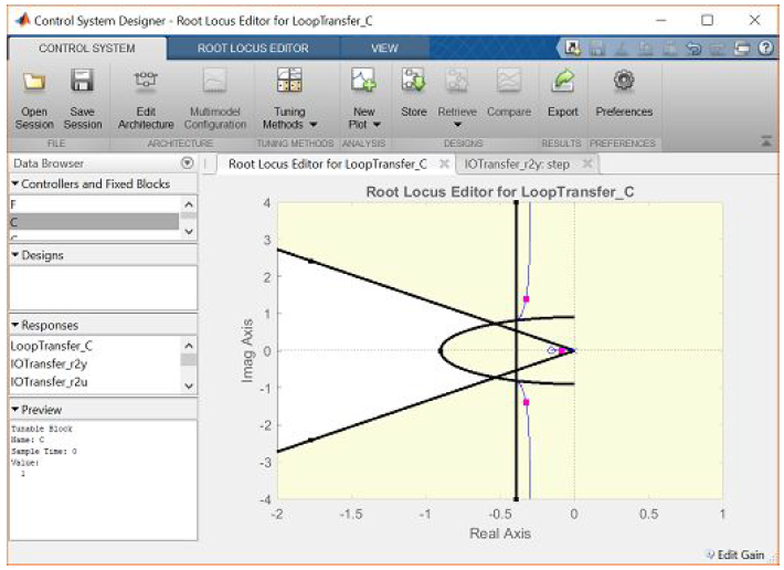
Lead Compensation:
We specifically need to shift the root locus more to the left in the complex plane to get it inside our desired region. We can do this is to employ a lead compensator.
The transfer function of a typical lead compensator is the following, where the zero has smaller magnitude than the pole, that is, it is closer to the imaginary axis in the complex plane.
We will place the pole further towards the left as we have to pull the root locus further towards the left.
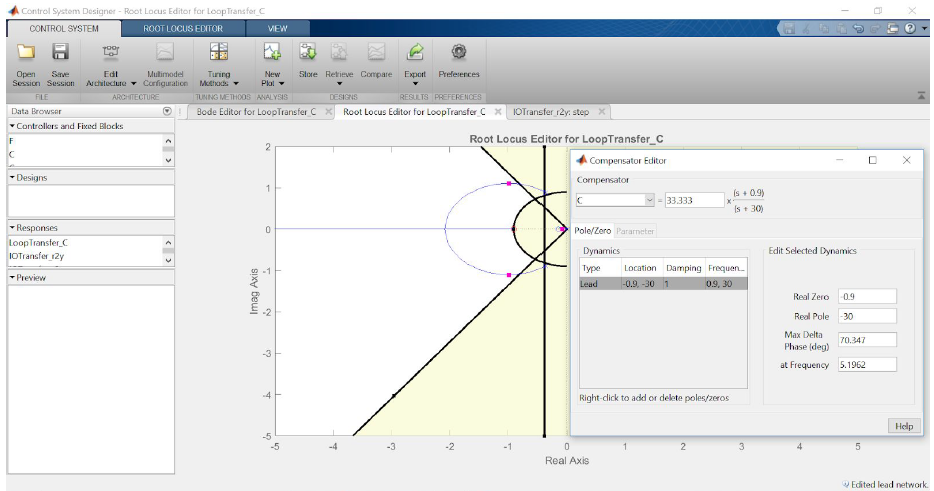
Now, varying the K value, we change the settling time and rise time to fall within our requirement. After changing the values of K, K=200 satisfies all of our requirements.
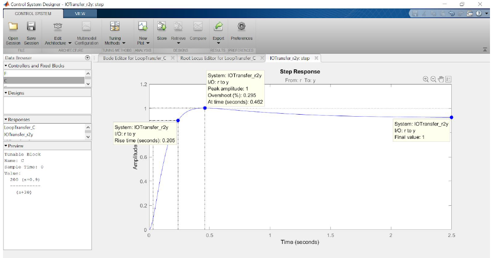
All of our design requirements are satisfied by this controller. This is our final Lead Compensator.
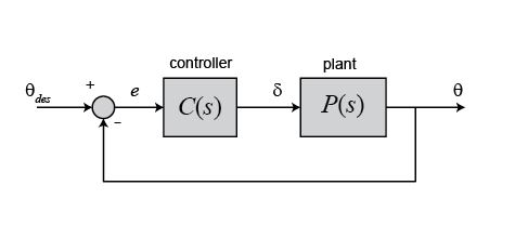
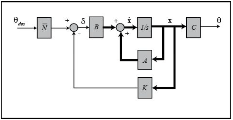
Control design via pole placement
The schematic of a full-state feedback control system is shown below (with D= 0).
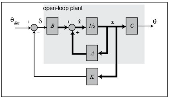
where,
K = control gain matrix
x = [α, q, θ] = state vector
θdes = reference (r)
δ= (θdes– Kx) = control input (u)
θ = output (y)
Referring back to the state-space equations at the top of the page, we see that substituting the state-feedback law δ = (θdes– Kx) for δ leads to the following.
x = ( A – BK)x Bθdes
θ= Cx
Based on the above, matrix A – BK determines the closed-loop dynamics of our system.
This feedback law presumes that all of the state variables in the vector x are measured, even though θis our only output. If this is not the case, then an observer needs to be designed to estimate the other state variables.
This process becomes more difficult if we have a higher-order system or zeros.
With a higher-order system, we can take advantage of Dominant Pole Phenomenon. The effect of zeros is more difficult to address using a pole-placement approach to control.
Another limitation of this pole-placement approach is that it doesn't explicitly take into account other factors like the amount of required control effort.
Linear quadratic regulation(LQR)
Linear Quadratic Regulator (LQR) method to generate the "best" gain matrix K, without explicitly choosing to place the closed-loop poles in particular locations.
This type of control technique optimally balances the system error and the
control effort based on a cost that the designer specifies that defines the relative
importance of minimizing errors and minimizing control effort.
In the case of the regulator problem, it is assumed that the reference is zero.
Therefore, in this case the magnitude of the error is equal to the magnitude
of the state.
For simplicity, we will choose the control weighted matrix (R) equal to 1 and the state-cost matrix (Q) equal to pC`C.
Employing the vector C from the output equation means that we will only
consider those states in the output in defining our cost.
In this case θ, is the only state variable in the output. The weighting factor (P) will be varied in order to modify the step response.
In this case R, is a scalar since we have a single input system.
Now, referring to the closed-loop state equations given above assuming a
control law with non-zero reference, δ = (θdes– Kx) , we can then generate the closed-loop step response.
Varying the value of p depending on the cost, we can vary the closed-loop step response. At p = 50, we get a satisfactory response regarding the settling time and response time. The graph is shown below –
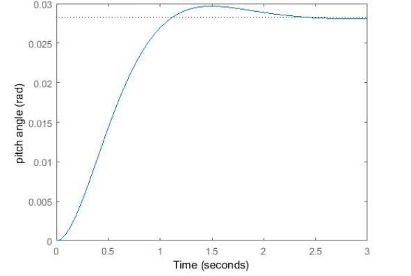
Examination of the above demonstrates that the rise time, overshoot, and settling time are satisfactory. However, there is a large steady-state error.
One way to correct this is by introducing a pre-compensator () to scale
the overall output.
Adding pre-compensation:
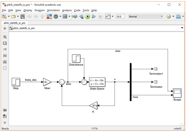
The full-state feedback system does not compare the output to the reference; instead, it compares all states multiplied by the control matrix (Kx) to the reference (see the schematic shown above).
Thus, we should not expect the output to equal the commanded reference. To obtain the desired output, we can scale the reference input so that the output does equal the reference in steady state.
This can be done by introducing a pre-compensator scaling factor called .
The basic schematic of our state-feedback system with scaling factor is shown below.
has been computed using the MATLAB function rscale.m .
After including the pre-compensator in the system, the modified step response looks like:
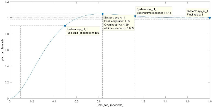
Now the steady-state error has been eliminated and all design requirements are satisfied.
The pre-compensator employed above is calculated based on the model of the plant and further that the pre-compensator is located outside of the feedback loop.
Therefore, if there are errors in the model (or unknown disturbances) the pre-compensator will not correct for them and there will be steady-state error.
We could have directly added an Integral Controller instead of a pre-compensator to resolve the error in steady-state value.
The tradeoff with using integral control is that the error must first develop before it can be corrected for, therefore, the system may be slow to respond.
The pre-compensator on the other hand is able to anticipate the steady-state offset using knowledge of the plant model.
A useful technique is to combine the pre-compensator with integral control to leverage the advantages of each approach.
This combined controller can be implemented by adding one more PI Controller or basically also involving this in the primary feedback controller.
We have implemented this model in the Simulink Model.
Digital Controller Design
The first step in the design of a digital control system is to generate a sampled-data model of the plant.
MATLAB can be used to generate this model from a continuous-time model using the c2d command. The c2d command requires three arguments: a system model, the sampling time (Ts) and the type of hold circuit. We will assume a zero-order hold (zoh) circuit.
In choosing a sample time, it is desired that the sampling frequency be fast compared to the dynamics of the system in order that the sampled output of the system captures the system's full behavior, that is, so that significant inter-sample behavior isn't missed.
One measure of a system's "speed" is its closed-loop bandwidth.
A good rule of thumb is that the sampling frequency be at least 30 times larger than the closed-loop bandwidth frequency which can be determined from the closed-loop Bode plot.
From the closed-loop Bode plot, the bandwidth frequency can be determined to be approximately 2 rad/sec (0.32 Hz).
Thus, to be sure we have a small enough sampling time, we will use a sampling time of 0.01 sec/sample.
The discrete-time state-space model shown below:
= [
y(k) = ] [0]
The schematic of a discrete full-state feedback control system is shown below,
where q-1 is the delay operator (not the aircraft's pitch rate q ). Note that it is assumed that D = 0.
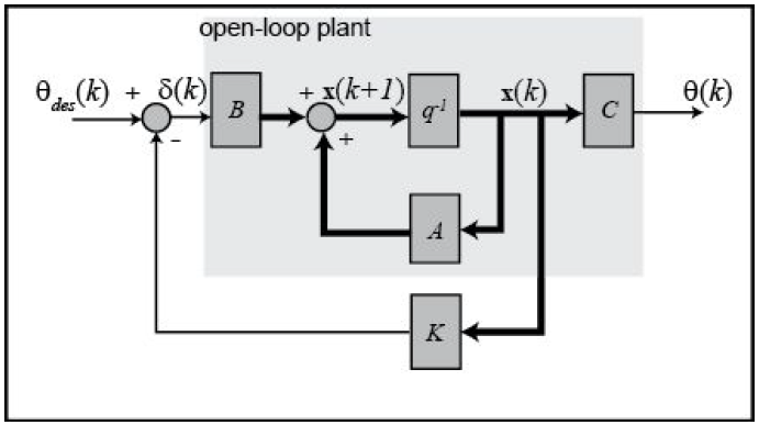
Discrete time system equations are:
x(k 1) = (A – BK) x (k) Bθdes(k)
θ(k) = Cx(k)
Linear quadratic regulation (LQR)
In this digital version, we will use the discrete version of the same LQR method.
This type of control technique optimally balances the system error and the control effort based on a cost that the designer specifies that defines the relative importance of minimizing errors and minimizing control effort.
Rest of the factors are the same as those in continuous time domain.
MATLAB Command dlqr which is the discrete-time version of the lqr command has been used. Both the cost matrices have been kept the same as that in continuous time domain.
Referring to the closed-loop state equations given above assuming a control law with non-zero reference, δ(k) = (θdes(k)– Kx(k)) , we can then generate the closed-loop step response.
Examining this step response, we will get a large steady-state error.
We have added a pre-compensator () to scale the overall output.
The user-defined function rscale.m to find because it is only defined for continuous systems.
The correct scaling by trial and error. After several trials, it was found that equal to 6.95 provided a satisfactory response.
After including this in the system, the modified step response looks like :
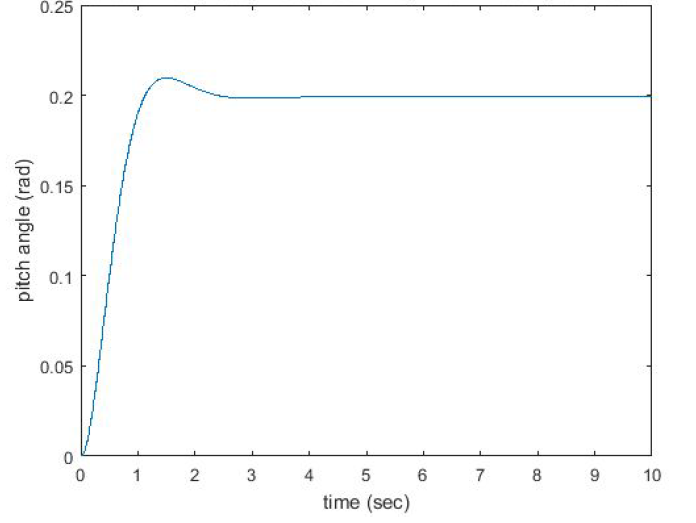
From this plot, we see that the factor eliminates the steady-state error. Now all design requirements are satisfied.
Simulink Modelling
Simulink modelling has been done to verify the plots of MATLAB and the results are well in sync.
But the main purpose of using Simulink was to model a disturbance and check the system robustness, especially with the use of a combined PI Control instead of just a pre-compensator which has been discussed below.
Continuing from the point of discussion of combining the pre-compensator and the proposed integral control in LQR, the drawback of using a pre-compensator like the one implemented above is that it is calculated on the basis of a model of the plant and is located outside of the feedback loop such that the output of the summing junction in the above model is no longer the true error.
Therefore, if there are errors in the model or an unknown disturbance, the pre-compensator will not correct for them and there will be steady-state error.
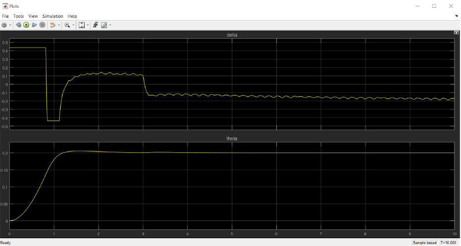
In order to investigate this phenomenon, we have added a disturbance to our model.
The disturbance is generated by a Step block with the Final value set to "0.2" and the Step time set to "3". The disturbance is modeled as entering the system in the same manner as the control input δ.
Running the simulation will generate a response like the one shown below.
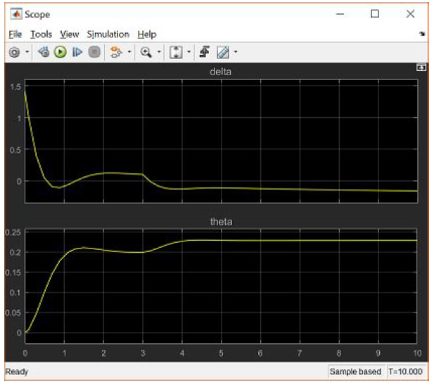
Inspection of the above plot demonstrates how the occurrence of the disturbance at a time of 3 seconds drives the system away from the desired steady-state value of 0.2 radians and the presence of the constant pre-compensator is not able to correct for the effect of the disturbance.
So we will add integral control also to it.
Model uncertainty is another source of error that should be considered. For example, if the "actual" system model had B a matrix equal to [0.232*1.4 0.0203*0.6 0]', then the controller K used above would lead to an unstable system.
This sort of result is not uncommon to controllers designed using a technique like the Linear Quadratic Regulator method.
This makes some sense in that the control gain K was designed only to minimize the resulting error and the required control effort; other goals, such as robustness to model uncertainty, were not considered in the design.
Automated PID tuning with Simulink:
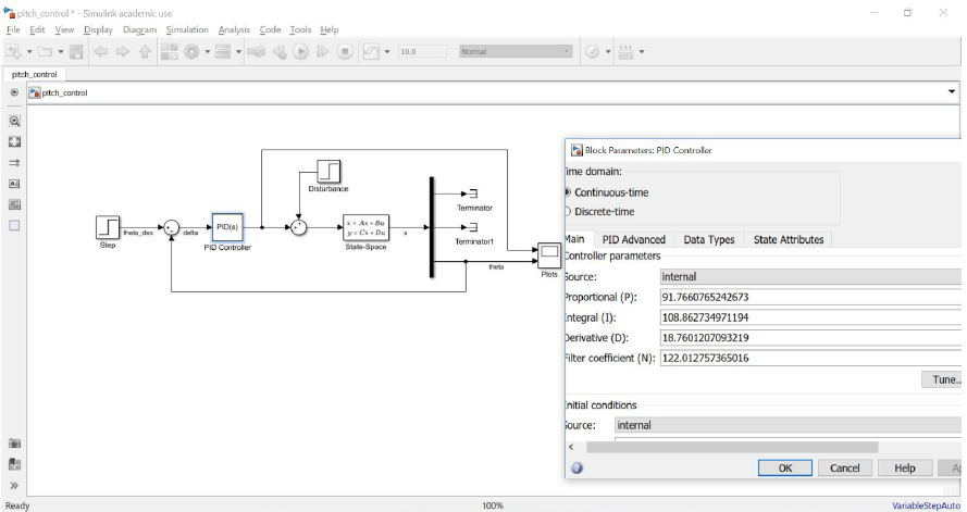
As mentioned above, adding integral control to our compensator can help to reduce the steady-state error that arises due to disturbances and model uncertainty.
We have implemented a PID controller assuming only the output θ is measured. Furthermore, we have used Simulink's built-in capabilities to automatically tune the PID controller.
The resulting model should appear as follows:
The step plot will look as follows:
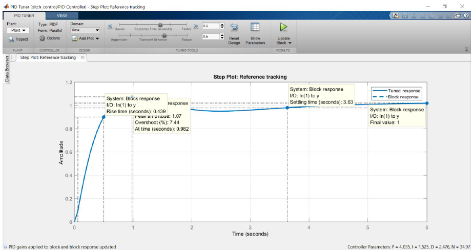
The performance of the controller (comparison of delta vs pitch):
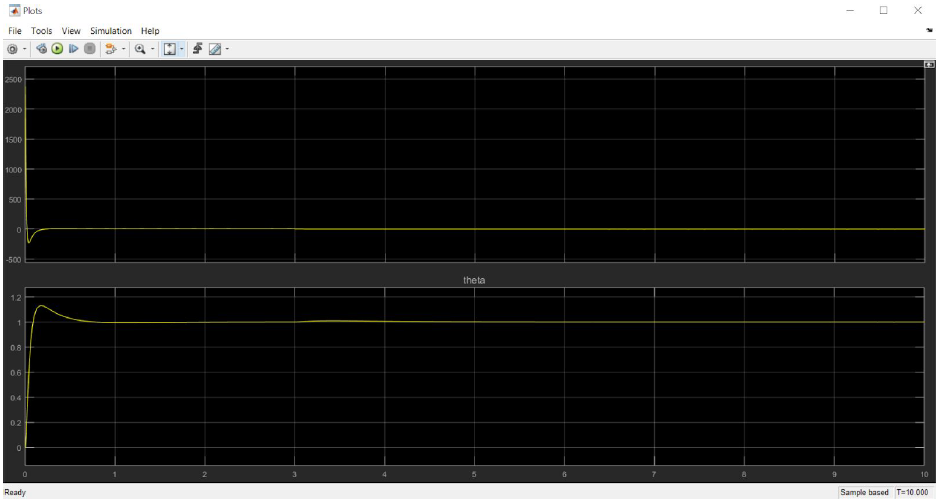
Thus, we can observe that the disturbance is corrected for in steady-state because the PID controller we are using includes an integral term.
In practice, it is likely that the elevator angle δ of the aircraft would be limited to something like that -25 degrees (-0.4363 rad) to 25 degrees (0.4363 rad).
To ensure that we don’t go beyond this limit, we have set the controller to saturate.
After choosing these options and running the simulation generates the following results which meet our requirements, even in the presence of the disturbance as shown below.
References
- Nurbaiti Wahid, “Self-Tuning Fuzzy PID Controller Design for Aircraft Pitch Control”, 2012.
- SiddharthGoyal, “Study of a Longitudinal Autopilot for Different Aircrafts”, 2007.
- Raghu Chaitanya. M. V, “Model Based Aircraft Control System Design and Simulation”, 2012.
- Ropert C. Nelson, “Flight Stability and Automatic Control”, 1989.
- Donald McLean, “Automatic Flight Control Systems”, 1990.
- Karl Johan A strom,” Control System Design”, 2002.
- Neil Kuyvenhoven, “PID Tuning Methods an Automatic PID Tuning Study with Mathcad”, 2002.
- TemeL, Semih YAĞLI and Semih GÖREN, “P, PD, PI, PID Controllers”, 2013.
- Michael Negnevitsky, “Artificial Intelligence a Guide to Intelligent Systems”,
- Narenathreyas, K., “Fuzzy Logic Control for Aircraft Longitudinal Motion”,
- Master Thesis, Faculty of Electrical Engineering, Department of Control Engineering, Czech Technical University, 2013.
- Roland Burns, “Advanced Control Engineering”, 2001.
- N. Wahid, N. Hassan, M.F. Rahmat and S. Mansor, “Application of Intelligent Controller in Feedback Control Loop for Aircraft Pitch Control”, 2011.
- Amir Torabi, Amin AdineAhari, Ali Karsaz and SeyyedHossinKazem,“Intelligent Pitch Controller Identification and Design”, 2013.
- A. B. Kisabo1, F. A. Agboola, C.A. Osheku1, M. A. L. Adetoro1 and A. A. Funmilayo, “Pitch Control of an Aircraft Using Artificial Intelligence”, 2012.
Conclusions
We have designed a PID Controller and a Lead Controller for controlling the pitch of an airplane.
We have used LQR to find the appropriate gain matrix.
We have discretized the system and then have performed all the analysis for the same.
We have worked on improving some of the common drawbacks of using pre-compensators in LQR, while also pointing out another drawback of this control technique, by using the Simulink model and during that, making our controller more robust (by testing it with the step-disturbance).
MATLAB Codes
% Aibek Ablay
% Department Of Electrical Engineering and Control Science | Nanjing Tech University
%File name: AirCraft_model.m
% This code will generate the open-loop transfer function of the
% longitudinal equations of motion for the aircraft, since Aircraft pitch
% is governed by the longitudinal dynamics
%*Important note: We will assume that the aircraft is in steady-cruise at
%constant altitude and velocity; thus, the thrust, drag,
%weight and lift forces balance each other in the x- and y-directions.
% We will also assume that a change in pitch angle will not change the speed
%of the aircraft under any circumstance
%** values are taken from the data from one of Boeing's commercial aircraft
%*** Thanks to http://ctms.engin.umich.edu
%**************************************************************************
%Transfer function:
s = tf('s');
pitch_angle = (1.151*s 0.1774)/(s^3 0.739*s^2 0.921*s)
t = [0:0.01:20];
step(0.15*pitch_angle,t);
axis([0 20 0 0.8]);
ylabel('pitch angle (rad)');
title('Open-loop Step Response');
rlocus(pitch_angle)
sys_CL = feedback(pitch_angle,1)
step(0.15*sys_CL);
ylabel('pitch angle (rad)');
title('Closed-loop Step Response');
p = 50;
Q = p*C'*C
R = 1;
[K] = lqr(A,B,Q,R)
Nbar = Rescale(A,B,C,D,K)
sys_CL = ss(A-B*K, B, C, D);
step(0.15*sys_CL)
axis([0 8 0 0.025])
ylabel('pitch angle (rad)');
title('Closed-Loop Step Response: LQR');
% State-space representation:
A = [-0.313 56.7 0; -0.0139 -0.426 0; 0 56.7 0];
B = [0.232; 0.0203; 0];
C = [0 0 1];
D = [0];
pitch_ss = ss(A,B,C,D)
User defined functions:
function[Nbar]=Rescale(a,b,c,d,k)
% Given the single-input linear system:
% x = Ax Bu
% y = Cx Du
% and the feedback matrix K,
%
% the function rscale(sys,K) or rscale(A,B,C,D,K)
% finds the scale factor N which will
% eliminate the steady-state error to a step reference
% for a continuous-time, single-input system
% with full-state feedback using the schematic below:
%
% /---------\
% R u | . |
% ---gt; N ---gt;() ----gt;| X=Ax Bu |--gt; y=Cx ---gt; y
% -| \---------/
% | |
% |lt;---- K lt;----|
error(nargchk(2,5,nargin));
% --- Determine which syntax is being used ---
nargin1 = nargin;
if (nargin1==2), % System form
[A,B,C,D] = ssdata(a);
K=b;
elseif (nargin1==5), % A,B,C,D matrices
A=a; B=b; C=c; D=d; K=k;
else error('Input must be of the form (sys,K) or (A,B,C,D,K)')
end;
% compute Nbar
s = size(A,1);
Z = [zeros([1,s]) 1];
N = inv([A,B;C,D])*Z';
Nx = N(1:s);
Nu = N(1 s);
Nbar=Nu K*Nx;
以上是毕业论文大纲或资料介绍,该课题完整毕业论文、开题报告、任务书、程序设计、图纸设计等资料请添加微信获取,微信号:bysjorg。
相关图片展示: